The Fast Fourier Transform One trick. From all-night to instant. Everywhere.

In 1805, Carl Friedrich Gauss worked out a clever shortcut for computing the orbit of an asteroid from a handful of observations. He wrote it up in a dense, old-fashioned Latin, set it aside, and never published it. The method sat in his notebooks, unread, for more than 150 years.

When James Cooley and John Tukey published essentially the same idea in 1965, they had no idea Gauss had beaten them to it. What they did know was that it was useful. Their four-page paper became one of the most cited in all of applied mathematics, and the algorithm it described, the Fast Fourier Transform, is now routinely listed among the most important of the twentieth century. The mathematician Gilbert Strang put it more strongly, calling it the most important numerical algorithm of our lifetime.

The rest of this post covers what the FFT actually computes, the trick that makes it fast, and the surprisingly wide range of places it turns up, from the app that names a song in a noisy bar to the wireless link carrying this page.

The version everyone uses today comes from Cooley, a mathematician at IBM's Watson Research Center, and Tukey, who held positions at Princeton and at Bell Labs. They developed it in 1964 on an IBM 7094, and the paper that made it famous, "An Algorithm for the Machine Calculation of Complex Fourier Series," appeared in Mathematics of Computation in April 1965. You will see both years cited: 1964 for the work, which is the date IEEE's milestone marks, and 1965 for the publication.

The backstory has a Cold War flavor. In 1963, at a meeting of President Kennedy's Science Advisory Committee, Tukey described the method to the physicist Richard Garwin, who was working on detecting Soviet nuclear tests from seismic recordings. Breaking those recordings into their frequencies was the slow step, and Tukey's shortcut was exactly what he needed. Garwin took the idea back to IBM and arranged for Cooley to implement it. Tukey himself was in no rush to write it up. He figured the trick was a simple observation that was probably already known, so Cooley took the lead, and they chose to publish in part so the method could not be patented and locked away.

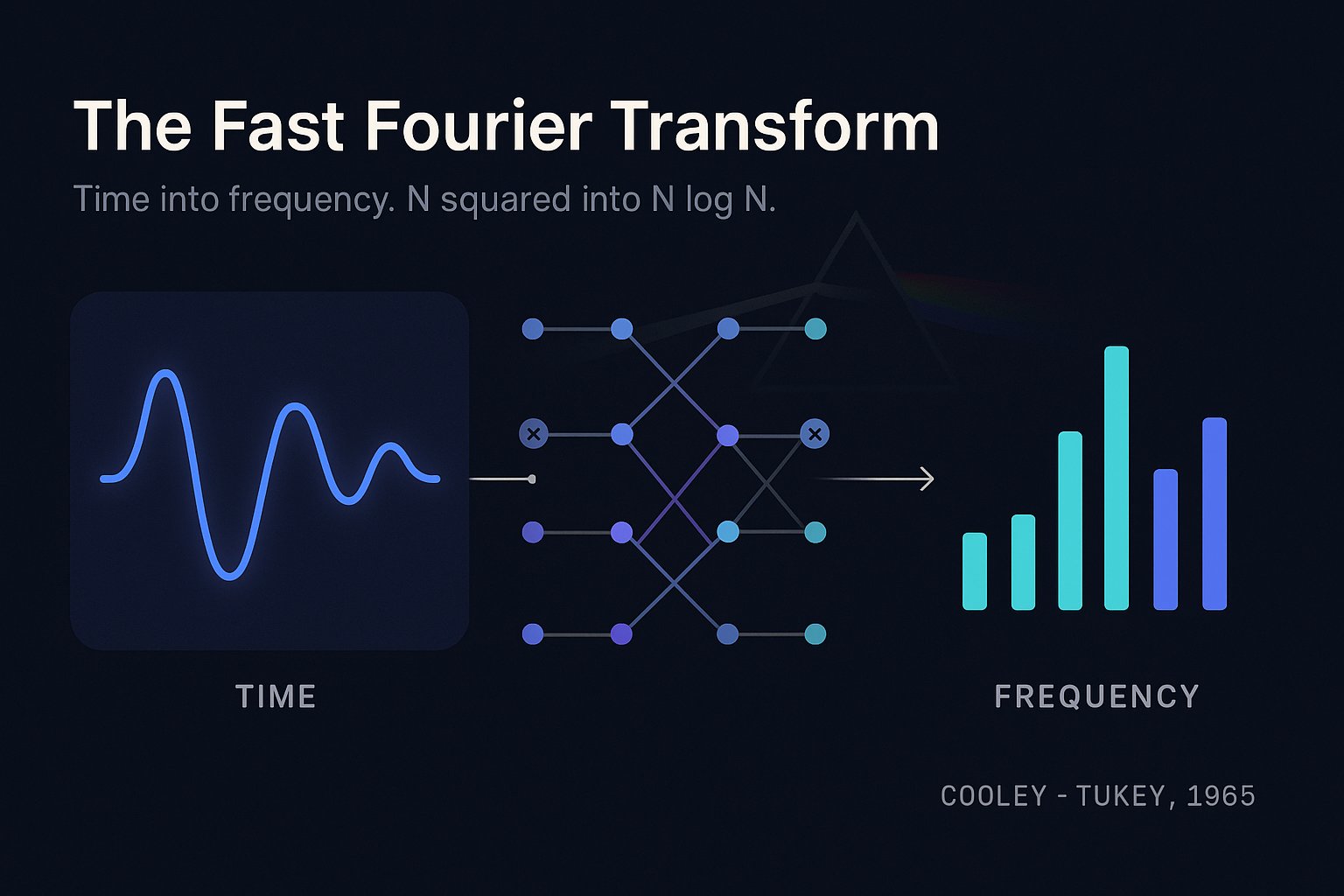
The core idea is that any signal can be rebuilt by adding up simple waves of different frequencies. A chord reaches your ear as one complicated pressure wave, but you know it is really several notes sounding at once. A Fourier transform is the procedure that takes the combined wave and recovers the individual notes, telling you how much of each frequency is present. It moves a signal from a description in time, its value at each instant, to a description in frequency, the mix of tones it contains. The old comparison is a prism splitting white light into its colors.

When the signal is a list of sampled numbers, say the readings a microphone takes thousands of times a second, you use the discrete version, the Discrete Fourier Transform, or DFT. Its definition is:

The takeaway matters more than the symbols. Each output value X[k] measures how strongly one frequency shows up in the signal, and you compute it by running across all N input samples and combining each with a rotating complex number.

The catch is the cost. One output value takes about N multiply-and-add steps, and there are N outputs, so computing the DFT directly takes on the order of N² operations. A single second of CD-quality audio holds roughly 44,000 samples, which puts N² near two billion operations for one second of sound. Scale that up to a whole song or a stack of medical images and the direct method stops being practical. For a long time, that cost was the reason frequency analysis stayed expensive.

The FFT computes the very same DFT, only far faster. It brings the cost down from around N² to around N log N. The gap is large. For a million points, the direct route needs something like a trillion operations, while N log N needs about twenty million, roughly fifty thousand times less work.

In practice that is the difference between a job you leave running overnight and one that finishes before you look up. That gap is the whole reason the FFT matters. Most of what fills the rest of this post, streaming video, digital wireless, real-time audio, medical imaging, depends on computing transforms fast enough to keep pace with data as it arrives, and at the brute-force N² cost, none of it would keep up.

The method is divide and conquer, and it rests on one observation. Split the input samples into the ones at even positions and the ones at odd positions. A little algebra shows that the DFT of the whole sequence can be written using only the DFT of the even samples, call it E, and the DFT of the odd samples, call it O:

One transform of size N has become two transforms of size N/2 plus some cheap arithmetic. The small multiplier in front is called a twiddle factor, and the pair of combine steps is called a butterfly, for the crossing shape it makes in a data-flow diagram. Notice that both outputs, X[k] and X[k+N/2], come from the same two pieces. That reuse is where the savings come from.

Here is the butterfly on its own. Two inputs come in on the left. The odd one is scaled by the twiddle factor. Then the same scaled value is added at the top and subtracted at the bottom, producing two outputs at once. The crossing of those two lines is the shape the operation is named for.

Then you do the obvious thing and split each half again, and again, until you reach transforms of a single point, which take no work at all. This is the same trick behind mergesort and binary search: each step cuts the problem in half, so a cost that looked like N² collapses to about N work at each of log₂ N levels, which multiplies out to N log N. Real implementations skip the recursion: they reorder the input once with a tidy index shuffle and then sweep through the levels in place, which runs very fast on actual hardware.

Stack those butterflies up and the whole 8-point FFT looks like this. The inputs enter on the left in a shuffled order, three stages of butterflies fire in turn, and the frequencies come out in order on the right. Three stages, because log₂ 8 = 3.

This is the Cooley-Tukey algorithm. The form above wants N to be a power of two, but there are relatives for other sizes and for awkward prime lengths. They all work the same way underneath, using structure and symmetry to skip repeated work.

This is where the math starts appearing in things you use every day. Some of these are easy to guess. Others are not obvious at all.

When you hold up your phone in a loud room and it names the song, you are watching the FFT run live. In the method Avery Wang described in 2003, Shazam cuts the incoming audio into short overlapping windows and runs an FFT on each one. Laid side by side, those results form a spectrogram, a picture of how the song's frequency content changes over time.

The part that makes it robust is what comes next. Rather than comparing whole spectrograms, which would fall apart with background noise, Shazam picks out the peaks, the points in time and frequency where the energy is locally strongest. Those peaks hold up well even when the room is noisy. It pairs nearby peaks and turns each pair into a small numeric fingerprint that encodes two frequencies and the time between them. Your phone sends a batch of these fingerprints to the server, which matches them against tens of millions of pre-indexed tracks. The whole thing sits on top of the spectrogram, which the FFT produces.

When you say "Hey Siri" or ask Alexa a question, an FFT runs before the device has any idea what you said. The usual first step in speech recognition is to chop the incoming audio into short overlapping windows and run an FFT on each one, which produces a spectrogram, the same sort of time-and-frequency picture Shazam builds. Speech carries most of its meaning in how energy is spread across frequencies and how that pattern shifts from moment to moment, so this view of the sound is far more useful to a recognizer than the raw waveform.

From there the system usually warps the frequencies onto a scale that matches human hearing and hands the result to a neural network, which turns the pattern into words. Wake-word detection works the same way and runs continuously on the device, listening for the spectral signature of "Alexa" or "Hey Siri" while everything else is ignored. So the front end of nearly every voice assistant and dictation feature is an FFT, converting sound into something a model can read.

MRI is a particularly striking case. A scanner does not measure your anatomy directly. Because of the way its magnetic gradients work, what it records is data in the spatial frequency domain, which physicists call k-space. To turn that into the cross-section a radiologist reads, the machine runs an inverse Fourier transform. The image of your knee is reconstructed from its frequencies.

There is also a purely mathematical use that surprises people. The convolution theorem, the fact that convolution becomes simple pointwise multiplication in the frequency domain, is why the FFT speeds up not just huge multiplications but large filtering jobs throughout signal and image processing. The same humble trick keeps turning up wherever something has to be done to every frequency at once.

For a clip of audio the FFT finishes in microseconds on a single core, and there is nothing to spread around. But some transforms are huge: a three-dimensional FFT over a cosmology simulation, a global climate model, a molecular dynamics run, or the data pouring out of a radio telescope array. Once the data outgrows one machine's memory, or one machine would simply be too slow, you have to split the work across many processors. That turns out to be hard, and the reason is instructive.

The trouble is that the FFT is global. Every output depends on every input, which is the whole point of breaking a signal into frequencies that run its full length. That is very different from, say, brightening every pixel in a photo, where you could hand each processor its own slice and never check back. With an FFT the processors have to trade data partway through, and there is no way around it. That communication, not the arithmetic, is what limits speed at scale. People call the FFT communication-bound: there is little math per byte moved, so the network between machines, rather than the processors, becomes the bottleneck.

How you carve up the data sets how far you can scale. The simplest scheme slices a 3D volume into flat slabs along one axis. The more scalable scheme cuts it along two axes into long thin pencils. Here is the difference.

Underneath all of this is an idea from David Bailey's 1989 work on FFTs for hierarchical and external memory, often called the four-step FFT, which reshapes even a single giant one-dimensional transform into a small two-dimensional problem, so each piece fits in one machine's memory and the transpose carries the communication.

It helps to separate two situations that both get called large-scale FFTs, because they could not be more different.

A lot of confusion clears up once you sort out which of the two you actually have. And you rarely write any of this yourself. On a single machine the long-standing standard is FFTW, the Fastest Fourier Transform in the West, and on GPUs it is NVIDIA's cuFFT. For clusters there is a whole ecosystem, including P3DFFT and FFTW's own distributed interface, and for GPU-based supercomputers there are libraries like heFFTe and multi-node tools such as cuFFTMp that handle the heavy all-to-all communication so researchers do not have to.

What makes the FFT satisfying is the gap between how plain it sounds and how much rides on it. Gauss used it to work out an asteroid's orbit and never bothered to publish. Cooley and Tukey revived it to listen for nuclear tests. Now it sits under medical scanners, wireless networks, and the app that names a song in a bar, doing the same humble job in each one: turning a calculation that would take all night into one that finishes before you notice.

“

Not bad for a trick its discoverers kept deciding was too obvious to bother with.

• Cooley, J. W. and Tukey, J. W., 1965. "An Algorithm for the Machine Calculation of Complex Fourier Series." Mathematics of Computation, 19(90), 297-301.
• Heideman, M. T., Johnson, D. H., Burrus, C. S., 1984. "Gauss and the History of the Fast Fourier Transform." IEEE ASSP Magazine, 1(4), 14-21.
• Danielson, G. C. and Lanczos, C., 1942. "Some improvements in practical Fourier analysis and their application to X-ray scattering from liquids." Journal of the Franklin Institute, 233(4), 365-380.
• Wang, A., 2003. "An Industrial-Strength Audio Search Algorithm." Proceedings of ISMIR. (The Shazam method.)
• Bailey, D. H., 1989. "FFTs in External or Hierarchical Memory." The Journal of Supercomputing, 4(1), 23-35. (The four-step FFT.)
• Frigo, M. and Johnson, S. G., 2005. "The Design and Implementation of FFTW3." Proceedings of the IEEE, 93(2), 216-231. See also fftw.org.