How LLM Inference Actually Works The map. Every later post zooms into one box.

Where we are in the stack: the whole thing. This post is the map. Every later post in the series zooms into one box on the diagram drawn here.

You hit an API endpoint with a prompt. A few hundred milliseconds later, words start streaming back. Most engineers stop being curious right there. The rest of this series is for the engineers who don't.

Before we can talk about KV caches, paged attention, or speculative decoding, we need an honest mental model of what an LLM is actually doing when it generates text. This post builds that model from the ground up. No prior GPU knowledge required. By the end you should be able to explain, to a colleague at lunch, why generating 500 tokens is fundamentally 500 sequential operations and why that single fact is the source of nearly every interesting engineering problem in modern inference.

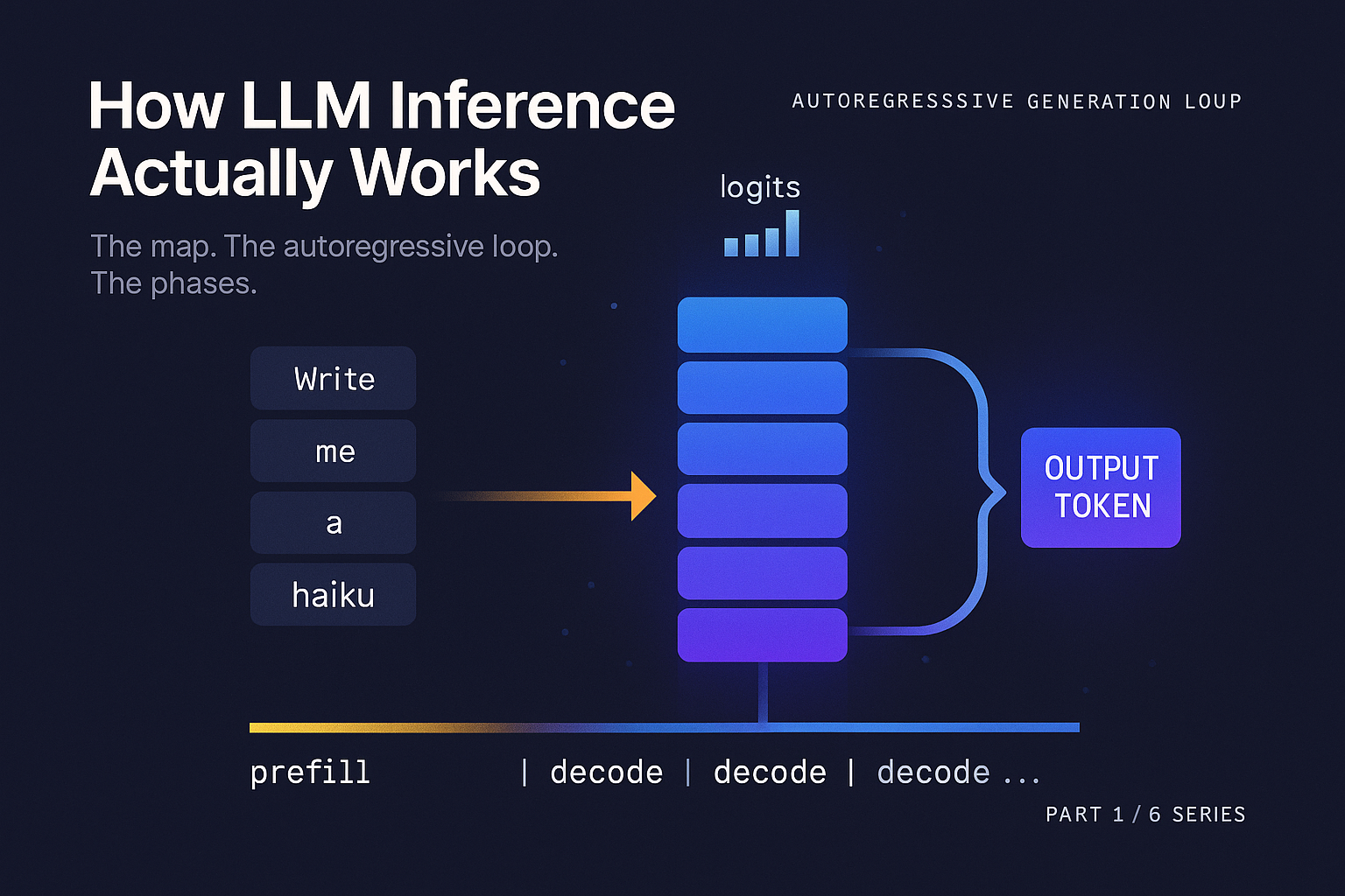
A language model generates text one token at a time. You feed in some tokens, the model produces a probability distribution over what the next token should be, you sample one token from that distribution, you append it to your input, and you run the whole thing again. Repeat until the model produces a special end token or you hit a length limit. Everything else in this series is a consequence of that loop.

We are not going to teach the transformer architecture from scratch. Hundreds of better tutorials exist. What we need is the smallest amount of mechanism that makes the rest of this series make sense.

When your text arrives at the model, a tokenizer breaks it into chunks called tokens. For a model like Llama 3, a token is on average about 3.5 to 4 characters of English text. Each token has an integer ID, and that ID indexes into an embedding table, producing a vector of numbers (typically 4096 or 8192 dimensions for modern models). One vector per token.

That sequence of vectors passes through a stack of identical layers. Llama 3 8B has 32 of these layers. Llama 3 70B has 80. GPT-3 had 96. Each layer has the same two sublayers in the same order:

• An attention block, where every token gets to look at every prior token and decide what information to pull from each.
• An MLP block (also called a feedforward block), where each token's vector is transformed independently of the others.

After the final layer, the vector at the last position is multiplied by a large matrix (the unembedding matrix, often tied to the embedding table) to produce a vector with one entry per token in the vocabulary. That vector is called the logits. Apply softmax to get a probability distribution. Sample. You now have your next token.

This architecture comes from Vaswani et al. 2017, "Attention Is All You Need". Eight years and many trillions of parameters later, the basic skeleton has barely changed. The improvements have mostly been in how the attention is computed, how the MLP is shaped, how positions are encoded, and how the whole thing is normalized. The crucial step is understanding how this core mechanism dictates the entire generation process, which is where the sequential nature of the autoregressive loop comes into play.

To generate token N, the model needs to know about tokens 1 through N minus 1. To generate token N plus 1, it needs to know about tokens 1 through N, which means it needs to have already produced token N. There is no way around this. Generation is sequential by construction.

This has a brutal consequence. A 500 token response is 500 sequential forward passes through the model. You cannot parallelize across the output dimension. You can throw an entire data center at one user's request and the latency floor will be set by how long it takes the model to produce a single token, multiplied by how many tokens you need.

This is why latency per token, not total compute, is the dominant cost in inference. To be precise, the computational cost for a single token generation step (decode) through the dense transformer model is roughly 2N FLOPs, where N is the parameter count, due to the matrix multiplications involved. It is also why almost every optimization we will discuss in this series exists. Speculative decoding tries to break the sequential dependency. Continuous batching tries to amortize the cost of each sequential step across many users. The KV cache exists so we don't have to recompute the whole prefix on every step. All of it is in service of fighting the autoregressive loop.

When a prompt arrives, the model has to process all of its tokens to figure out where to start generating. This phase is called prefill. The prompt might be 8 tokens or 8000 tokens, but they are all known up front. The model can process them in parallel. One forward pass, all prompt tokens in flight at once, lots of matrix multiplication, GPU running at full tilt.

Once prefill is done, the model emits the first new token. Now it has to emit the second. It has to emit the third. Each of these steps is a separate forward pass, but with only one new token to compute. This phase is called decode. The matrices being multiplied are now very tall and very thin (one row instead of thousands), which means the math gets done in microseconds but the GPU spends most of its time waiting on memory.

The asymmetry is dramatic. Prefill is compute bound. The GPU is doing real math, the FLOPs counter goes brrr, and a longer prompt gets prefilled in roughly linear extra time (up to the point where attention's quadratic cost kicks in). Decode is memory bandwidth bound. To produce one token you have to read every weight in the model out of VRAM. The model can be 16 GB or 160 GB, and that read sets the floor on how fast tokens can come out.

This split is why your TTFT (time to first token) and your ITL (inter token latency) feel like two different problems. They are two different problems. TTFT is a prefill problem. ITL is a decode problem. We will come back to both in Part 5.

A useful frame for the whole series is that GPU inference is a constant negotiation between three resources.

Make the bandwidth point concrete, because it is the one that surprises people. An NVIDIA H100 has roughly 3.35 TB/s of HBM3 memory bandwidth. A 70 billion parameter model stored in FP16 takes 140 GB. To read every weight once takes at minimum 140 / 3350, or about 42 milliseconds. That is your hard floor for a single decode step on one H100, regardless of how clever your kernels are.

You cannot make tokens come out faster than your bandwidth allows. (In practice it gets worse, because you also have to read the KV cache, but that is a Part 4 problem.) The compute side tells a different story. That same H100 can do about 1979 TFLOPS in FP16 with sparsity, but its dense FP16 throughput is closer to 500 TFLOPS. A single decode step for a 70B model is roughly 140 GFLOPs of math (two FLOPs per parameter per token). At 500 TFLOPS, that is about 0.28 milliseconds of pure compute. Even so, this is still over 150 times less than the memory read time.

So during decode, the GPU is computing for less than half a percent of the time and waiting on memory for the rest. This is the fundamental reason batching exists. If you can batch 32 users into one forward pass, you read the weights once and amortize the bandwidth cost across 32 tokens. The compute goes up 32x, but compute was free anyway. The math is the same, but you got 32x the throughput.

Williams, Waterman, and Patterson formalized this kind of analysis as the roofline model in their 2009 paper of the same name. We will use it explicitly in Part 3, but the intuition is already here: every operation has an arithmetic intensity (FLOPs per byte loaded), and your performance is bounded by whichever roof, compute or bandwidth, you hit first.

Let's walk one real request through the system. You send "Write me a haiku about autumn" to a Llama 3 8B model running on a single H100.

Step 1: Tokenization. Your string becomes a list of integers. The Llama 3 tokenizer would turn this into roughly 8 tokens. Cost: microseconds, on the CPU.

Step 2: Prefill. Those 8 token IDs are sent to the GPU. The model runs one forward pass with all 8 tokens in parallel. For an 8B model in BF16, this involves reading about 16 GB of weights and doing roughly 8 × 16 = 128 GFLOPs of math (per the rule of thumb that one token through a dense model is about 2N FLOPs where N is the parameter count). On an H100 this takes a handful of milliseconds, dominated by attention compute and matmul throughput. The output is a logit vector of size 128,256 (Llama 3's vocab size) for the last position. Sample from it. You get a token, let's say "Crimson".

Step 3: First decode step. The token "Crimson" gets its embedding looked up and goes through the model. But here is the trick: the model does not reprocess "Write me a haiku about autumn". It cached the intermediate state from prefill. (Specifically, the keys and values inside each attention layer. The K and V tensors. The KV cache. We'll do this in detail in Part 4.) So the decode step only has to compute one token's worth of new state, while reading the cached state for the prior 8 tokens. The forward pass for this single token is now memory bound: read 16 GB of weights, read the KV cache, do a tiny amount of math, produce the next logits. Sample. Get "leaves".

Step 4: Repeat. "drift" → "down" → "/" → "Whisper" → "of" → "the" → ... and so on until either an EOS token shows up or you hit your max_tokens limit. Each step is another full read of the model weights.

Step 5: Detokenization. The integer IDs get turned back into a string. The string streams back to you.

The whole haiku might be 30 tokens. That is one prefill of 8 tokens and 30 decode steps. The prefill takes maybe 5 milliseconds. Each decode step takes maybe 8 milliseconds. Total: about 245 milliseconds. Your TTFT is about 13 milliseconds (prefill plus first decode). Your average ITL is about 8 milliseconds.

These numbers are rough, but they are within a small factor of what a real serving system delivers in 2026. And every one of them is a target for the optimizations in the rest of this series.

If you are going to talk to a serving team or evaluate an inference vendor, four metrics carry most of the weight.

The tension between these metrics is the whole game. Every serving decision is a point on a multi-dimensional tradeoff surface.

Bigger batches help throughput, hurt TTFT. Speculative decoding helps ITL, costs compute. KV cache quantization helps capacity, hurts a little accuracy. Zhong et al. introduced the goodput framing clearly in the DistServe paper (2024), and it has become the standard way to evaluate serving systems honestly.

You now have an accurate mental model of inference. You know that generation is sequential. You know that prefill and decode are two completely different workloads. You know that three resources (compute, bandwidth, capacity) constrain everything and that decode is almost always memory bound.

The rest of the series is a tour through the stack, with each post owning one component.

Part 2 asks how the model gets onto the GPU in the first place. What is in a safetensors file, why naive loaders are slow, and what GPUDirect Storage actually does.

Part 3 opens up the forward pass. We will walk one token through the model layer by layer, count FLOPs and bytes, and use the roofline model to explain why FlashAttention was such a big deal.

Part 4 is the KV cache. Sizing it, fragmenting it, paging it, quantizing it, sharing it across requests.

Part 5 turns one model into a service. Continuous batching, chunked prefill, prefill / decode disaggregation, and speculative decoding.

Part 6 is quantization end to end. Weights, activations, and KV cache, and how the choices interact.

You now know what inference is. The rest of the series is about why doing it efficiently is hard, and what production systems actually do about it.

• Vaswani et al., 2017. "Attention Is All You Need." arXiv:1706.03762.
• Williams, Waterman, Patterson, 2009. "Roofline: An Insightful Visual Performance Model for Multicore Architectures." Communications of the ACM.
• Zhong et al., 2024. "DistServe: Disaggregating Prefill and Decoding for Goodput-optimized LLM Serving." arXiv:2401.09670.
• Touvron et al., 2023. "Llama 2: Open Foundation and Fine-Tuned Chat Models." arXiv:2307.09288. (Context on modern transformer choices.)
• Kaplan et al., 2020. "Scaling Laws for Neural Language Models." arXiv:2001.08361. (Background on the 2N FLOPs per token heuristic.)