Inside the Forward Pass One token. Every layer. Where the FLOPs and bytes go.

Where we are in the stack: one token, one trip through the model. The weights are loaded (Part 2). We have not yet talked about caching anything (Part 4) or serving multiple requests (Part 5). This post is about the computation itself.

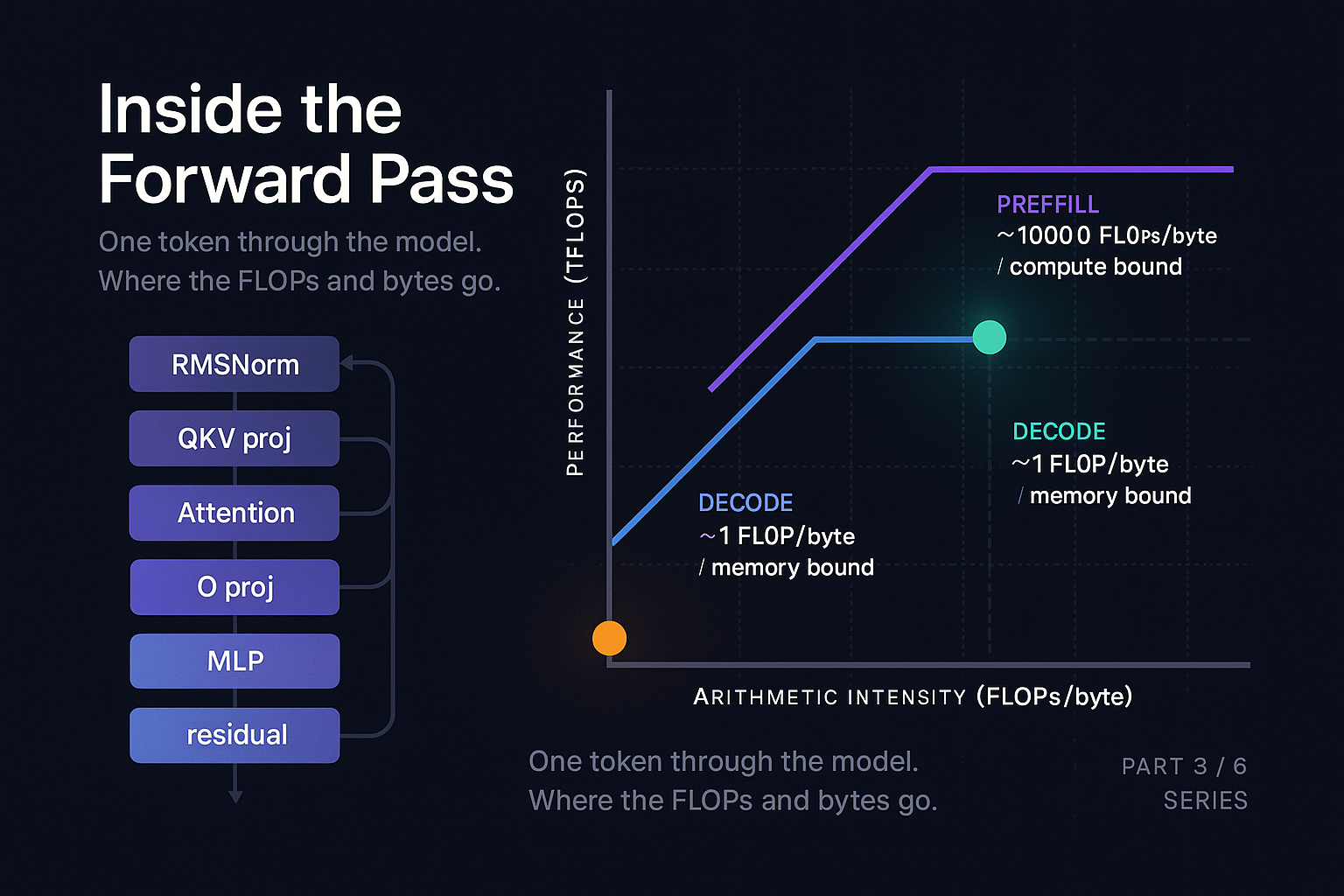
In Part 1 we said decode is memory bandwidth bound and prefill is compute bound. This post is where we earn those claims. We will walk a token through every layer of a transformer, count the FLOPs and the bytes, plot it on a roofline diagram, and use that to explain why FlashAttention was such a big deal and why fused kernels matter so much for production serving.

We will not derive the transformer from scratch. The Vaswani et al. 2017 paper is short and you should read it. What we will do is treat the forward pass as a sequence of operations and ask, for each, where the time goes.

A modern decoder-only transformer (Llama, Mistral, Qwen, GPT-style) repeats the same layer N times. Llama 3 8B uses 32 layers. The layer looks like this:

x = input          # shape: [batch, seq, d_model]
y = RMSNorm(x)
q, k, v = QKV projections of y
attn_out = Attention(q, k, v)
x = x + O_projection(attn_out)
y = RMSNorm(x)
mlp_out = MLP(y)
x = x + mlp_out

The + operations are the residual connections, which let gradients flow during training and (more relevant for us) let the model preserve information across layers. RMSNorm is a simplification of LayerNorm from Zhang and Sennrich, 2019. Most modern open models use it because it is cheaper than LayerNorm and works just as well.

The two big computational chunks are the attention block and the MLP. Everything else is comparatively small.

Let's pin down the numbers using Llama 3 8B as our reference. Each transformer layer has:

Total per layer: about 218 M parameters. Multiply by 32 layers: 6.96 B. Add the embedding table (128,256 * 4096 = 525 M, but tied to the output projection so we don't double count) and a final RMSNorm. Round up: 8 B. Hence the name.

Now FLOPs. For a single token (batch=1, seq=1) flowing through one layer in the decode case, each matmul of shape [1, A] @ [A, B] is 2*A*B FLOPs (one multiply, one add per output element).

• Q projection: 2 × 4096 × 4096 = 33.6 M FLOPs
• K projection: 2 × 4096 × 1024 = 8.4 M
• V projection: 8.4 M
• O projection: 33.6 M
• MLP gate, up, down: 3 × 2 × 4096 × 14336 = 352 M
• Attention (S = 1000): ~16 M (QK dot product + AV product)

Total per layer per token in decode: roughly 450 M FLOPs (dominated by MLP, then by projections; attention is tiny in absolute terms for short-to-medium contexts).

Across 32 layers: about 14.4 G FLOPs per token. The Kaplan et al. (2020) rule of thumb says one forward pass through a dense model costs about 2N FLOPs per token where N is the parameter count. For 8B params that gives 16 G FLOPs. The two numbers agree to within rounding error.

On an H100, which can do about 989 TFLOPS dense in BF16, 14.4 G FLOPs is 14.6 microseconds of pure compute time.

Now bytes moved. In decode, to process one token through one layer, we have to read:

• All weights for that layer: 218 M parameters × 2 bytes (BF16) = 437 MB
• Plus the KV cache for all prior tokens, which we will cover in Part 4

Across 32 layers: 14 GB of weights, plus KV cache reads.

H100 has 3.35 TB/s of HBM3 bandwidth. 14 GB takes 14 / 3350 = 4.2 milliseconds to read.

Here is the punchline. To produce one token in decode mode:

• Compute time: 14.6 microseconds
• Memory read time: 4.2 milliseconds

The ratio is 287. The GPU is computing for 0.35% of the time and waiting for memory for 99.65% of the time.

This is the roofline analysis. Arithmetic intensity is FLOPs per byte loaded. For decode of an 8B model in BF16, the intensity is 14.4 GFLOPs / 14 GB = about 1 FLOP per byte. The H100's "ridge point" (where compute and bandwidth balance) is at about 295 FLOPs per byte (989 TFLOPS / 3.35 TB/s). We are two orders of magnitude below the ridge. We are deeply memory bound.

For prefill, the math changes. If we process a batch of B tokens in parallel through the same layer, the weights still get read once, but the compute scales by B. Arithmetic intensity becomes B. Once B exceeds about 295 (whether through actual prompt length or batching multiple requests), we cross the ridge into compute bound territory. A 1000 token prompt prefill is firmly compute bound, which is why prefill saturates the GPU and decode does not.

A kernel, in CUDA parlance, is a function that runs on the GPU. Every operation you do in PyTorch (a matmul, an addition, a softmax) launches a kernel. Launching a kernel has overhead: the CUDA driver has to set up the launch, push it onto a stream, and wait for it to start executing on the device. The overhead per launch is small (microseconds) but it adds up.

More importantly, every separate kernel reads its inputs from VRAM and writes its outputs to VRAM. Two kernels chained together read the same intermediate tensor twice (once written by the first, once read by the second).

A fused kernel combines multiple operations into one. The intermediate lives in registers or shared memory and never round trips through HBM.

PyTorch 2.0's torch.compile is largely about automatic kernel fusion. It traces your forward pass, builds an IR, and uses TorchInductor (often emitting Triton kernels) to generate fused kernels. For inference workloads the speedups are often 2x to 3x on memory bound ops with no code changes from the user.

In production serving, custom fused kernels go further. TensorRT-LLM ships hand-tuned kernels for the tall, thin matrices of decode. vLLM has a growing Triton kernel library. SGLang composes its own. The gap between "vanilla PyTorch" and "production inference engine" on the same hardware is typically 3x to 10x, almost all of it from kernel quality.

Attention is the most interesting kernel in the model and the one most aggressively optimized. Naive attention does:

S = matmul(Q, K.T)     # shape [seq, seq], potentially huge
P = softmax(S)        # same shape
O = matmul(P, V)       # shape [seq, head_dim]

The intermediate S and P matrices are quadratic in sequence length. For an 8000 token context with 32 heads, that is 8000 × 8000 × 32 × 2 bytes = 4 GB per layer of intermediates stored in HBM. Read and written. Across 32 layers. The bandwidth cost dominates everything.

Dao et al. (2022) introduced FlashAttention with a brilliant observation: you do not have to materialize the full attention matrix. You can tile the computation, processing one block of queries against streaming blocks of keys and values, accumulating the output incrementally. Softmax can be computed incrementally if you track a running maximum and sum (the online softmax of Milakov and Gimelshein, 2018). The full attention matrix never exists in HBM, only blocks of it exist briefly in SRAM (the GPU's on-chip cache).

The numerical results are dramatic. FlashAttention is 2x to 4x faster than naive PyTorch attention on long sequences, uses far less memory, and is more numerically stable. Within a year it became the default in every serious inference engine.

FlashAttention-2 (Dao, 2023) improved parallelization. FlashAttention-3 (Shah et al., 2024) added Hopper-specific optimizations (asynchronous TMA copies, FP8 support, warpgroup matmul instructions) and pushed attention to 75% utilization in standard configurations, reaching 840 TFLOPs/s in BF16 (about 85% of the H100's dense peak) and 1.3 PFLOPs/s in FP8.

Look back at Llama 3 8B's hyperparameters. It has 32 query heads but only 8 key/value heads. This is Grouped Query Attention (Ainslie et al., 2023). Every group of 4 query heads shares one set of K and V heads.

The motivation is exactly the bandwidth concern we have been discussing. In decode, the KV cache has to be read on every forward pass, and its size scales with n_kv_heads. Cutting kv heads by 4x cuts the KV cache memory and bandwidth by 4x. The quality cost is small (Llama 3 70B uses 8 kv heads with 64 query heads and matches dense-attention models on benchmarks).

A more aggressive variant is Multi-Query Attention (Shazeer, 2019) which uses a single shared K and V head. PaLM and the original Falcon used this. The accuracy tradeoff was more visible, which is why GQA with 8 kv heads emerged as the sweet spot.

Let's trace one decode step end to end for Llama 3 8B, assuming a context of 1000 prior tokens already in the KV cache. For each of 32 layers:

This matches the Counting Bytes section above: 14 GB of weights per token at 3.35 TB/s gives 4.2 ms in pure bandwidth, plus output projection and attention KV reads bringing the idealized total to about 5.3 ms. Real world is typically 5 to 10 ms because of kernel launch overhead, suboptimal kernels, and KV cache reads that scale with context length. But the rough shape is right.

If you swap the model for Llama 3 70B (140 GB instead of 16 GB of weights), the per-step time goes up roughly 8x to 9x. Bandwidth bound, as predicted.

Three practical implications fall out of the roofline view.

Decode is bandwidth bound. Prefill is compute bound. The roofline model explains both and lets you predict the impact of optimizations before you implement them. FlashAttention is a worked example of how to escape a bandwidth bound regime by keeping intermediates in fast memory. Kernel fusion in general matters because every kernel boundary is a round trip through HBM.

In Part 4 we will look at the one tensor we have been suspiciously quiet about: the KV cache. It is small in relative terms but it has properties that wreck naive memory management.

• Vaswani et al., 2017. "Attention Is All You Need." arXiv:1706.03762.
• Williams, Waterman, Patterson, 2009. "Roofline: An Insightful Visual Performance Model for Multicore Architectures." Communications of the ACM, 52(4).
• Zhang and Sennrich, 2019. "Root Mean Square Layer Normalization." arXiv:1910.07467.
• Dao et al., 2022. "FlashAttention: Fast and Memory-Efficient Exact Attention with IO-Awareness." NeurIPS 2022. arXiv:2205.14135.
• Dao, 2023. "FlashAttention-2: Faster Attention with Better Parallelism and Work Partitioning." arXiv:2307.08691.
• Shah et al., 2024. "FlashAttention-3: Fast and Accurate Attention with Asynchrony and Low-precision." arXiv:2407.08608.
• Shazeer, 2019. "Fast Transformer Decoding: One Write-Head is All You Need." arXiv:1911.02150.
• Ainslie et al., 2023. "GQA: Training Generalized Multi-Query Transformer Models from Multi-Head Checkpoints." arXiv:2305.13245.
• Milakov and Gimelshein, 2018. "Online normalizer calculation for softmax." arXiv:1805.02867.
• Kaplan et al., 2020. "Scaling Laws for Neural Language Models." arXiv:2001.08361.