Where we are in the stack: above the model, where requests meet hardware. We know how a single forward pass works (Part 3) and how the KV cache is managed (Part 4). Now we turn one model into a service that handles thousands of users at once.
A model is a function. A service is something that takes a stream of requests, decides what to do with them, runs them on a finite pool of GPUs, and sends responses back. Going from the first thing to the second is most of what an inference engine actually does.
This post is about the scheduling and batching layer. It is also where the engineering creativity in this series peaks, because the constraints (Part 1's three resources, Part 3's roofline, Part 4's KV cache management) come together and produce a small number of techniques that have transformed inference economics.
Why one request at a time wastes the GPU
Recall from Part 3: decode is bandwidth bound. To produce one token from Llama 3 8B, you read all 16 GB of weights. That takes about 5 ms on an H100. The math itself takes about 15 microseconds. Three hundred times less.
If you serve one user at a time, the GPU spends 99.7% of decode time waiting on memory. You bought a fifty thousand dollar accelerator and you are using less than half a percent of its compute.
1 token per 5 ms forward pass
32 tokens per 5 ms forward pass
If you serve 32 users in the same forward pass, you still read the weights once but now the math is done for 32 tokens. The math takes 32 × 15 microseconds = 0.48 ms. Still well under the 5 ms bandwidth time. Throughput is 32 tokens per 5 ms instead of 1 token per 5 ms. You are now using 10% of compute and the cost per token has dropped by 30x or so.
This is why batching is the single most important throughput lever in LLM serving. It is also why batching is hard, because requests do not arrive in lockstep.
Static batching, and why it falls apart
The simplest scheme: collect N requests, run them through the model in lockstep, return all answers. The problem is that requests have different prompt lengths and different output lengths. If you batch 32 requests together, and one user wants 2000 tokens but the other 31 want 50 tokens, then 31 of your batch slots sit idle for the 1950 extra decode steps that the long user keeps the batch alive. Your effective utilization collapses.
You can pad up to a fixed length and accept the waste. You can sort requests by expected length, but you do not know the actual length until generation ends. You can chunk into many small batches, but small batches lose the very benefit you batched for.
Static batching was how research code worked. It was never going to fly for production serving. Until 2022, though, it was largely how production worked too. The technique that changed everything came from a group at Seoul National University.
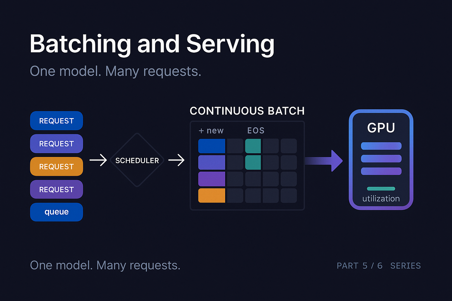
Continuous batching
Yu et al. introduced iteration-level scheduling in the Orca paper (2022). The idea is so clean in hindsight that you wonder why it took five years after attention came out.
Instead of batching at the request level (decide on a batch, run it to completion, decide on the next batch), batch at the iteration level. Every forward pass is its own scheduling decision. After each step:
- Sequences that finished (EOS or max length) drop out
- New requests waiting in the queue can be added to the next batch
- The batch dimension is dynamic, changing every step
This is called continuous batching or in-flight batching. The result is that the GPU is constantly running a roughly full batch, with no waiting-for-the-longest-request waste. Throughput improvements on real workloads were typically 2x to 4x over static batching, sometimes much more on long tail traffic patterns.
The implementation gets fiddly. Each sequence in the batch is at a different position in its generation, so the attention kernel has to handle a "ragged" batch where each row has a different effective length. The KV cache for each sequence lives at a different location. New requests entering the batch need their prefill done while existing requests are doing decode, which leads to the next problem.
Mixing prefill and decode: chunked prefill
There is a fundamental tension in continuous batching. Decode steps are short (single tokens, lots of users at once) and bandwidth bound. Prefill steps are long (many tokens, single user) and compute bound. If you mix them naively, a prefill step blocks all the decode steps in the batch from completing, hurting their ITL.
Agrawal et al. introduced chunked prefill in their SARATHI paper (2023). The idea: split a long prefill into smaller chunks, and run each chunk piggybacked with the decode work for other sequences in the same forward pass. If your prefill is 4000 tokens, you might break it into 8 chunks of 500 tokens. Each forward pass processes 500 prefill tokens for the new sequence plus the decode tokens for the dozens of in-flight sequences.
The benefit is that decode steps maintain steady cadence while the new sequence prefills incrementally. TTFT for the new user goes up slightly (the prefill is now spread across multiple steps) but ITL for existing users does not spike.
Chunked prefill is now standard in vLLM, TensorRT-LLM, and SGLang. The chunk size is tunable. Smaller chunks favor decode ITL; larger chunks favor TTFT. Most production systems sit around 512 to 2048 tokens per chunk.
Disaggregation: separating prefill and decode
The chunked-prefill solution to mixing prefill and decode is good but not perfect. Even with small chunks, the two workloads have fundamentally different hardware preferences. Prefill saturates compute and gets little benefit from extra GPUs (compute scales with FLOPs which scales with parameters and tokens). Decode is bandwidth bound and benefits hugely from being spread across more GPUs (you can split the weight reads across more memory channels).
The natural conclusion is to run them on separate pools of GPUs. Prefill / decode disaggregation does exactly that.
Prefill Pool
NVLink / IB
Decode Pool
A request arrives at a prefill worker, which runs prefill and produces the KV cache for the full prompt. That KV cache then gets transferred to a decode worker, which runs the autoregressive decoding. The two pools can be sized independently. Prefill pools can run on cheaper GPUs (or fewer of them) since they are compute bound and benefit from large batches. Decode pools want lots of HBM bandwidth per parameter.
The challenge is the KV cache transfer. Moving a few GB of KV cache between GPUs over NVLink or InfiniBand is not free. Splitwise (Patel et al., 2024) and DistServe (Zhong et al., 2024) both worked through the design tradeoffs. DistServe reported 4x to 7x higher goodput (throughput within SLO) compared to coupled serving on long-context workloads.
As of 2026, disaggregation is the cutting edge of production serving but not yet universal. It requires good interconnect (NVLink between prefill and decode hosts, or fast networking) and orchestration that hides the cross-tier handoff from latency. NVIDIA's Dynamo (announced 2025) is built around disaggregation. SGLang has experimental support. Most simple deployments still run coupled.
Speculative decoding
The autoregressive loop is the fundamental latency constraint. Each new token requires reading all the weights. Speculative decoding tries to break this constraint by checking many candidate tokens at once.
The setup: you have your big target model, the one whose outputs you want. You also have a small draft model (typically 10x to 100x smaller). The draft model is fast but less accurate. The protocol:
- Draft generates K tokens. K is typically 3 to 8. Fast because the draft is small.
- Target verifies in one forward pass. Single pass through the target with all K candidates as input.
- Compare. Accept tokens until first disagreement; take target's choice at that position.
- Repeat.
Crucially, step 2 is a single forward pass through the target model, even though it produces up to K accepted tokens. The cost is one weight read instead of K. If the acceptance rate is high (the draft and target agree often), you can get 2x to 4x speedups.
The paper that made this rigorous is Leviathan et al. (2023), along with Chen et al. (2023) from DeepMind. Both papers showed how to do this exactly: with a small math trick (rejection sampling against the target's true distribution), you get tokens that are statistically identical to what the target would have produced on its own. The speedup is free in terms of output quality.
Variants have proliferated. Medusa (Cai et al., 2024) replaces the draft model with additional output heads on the target itself. EAGLE (Li et al., 2024) uses a small autoregressive head on the target's hidden states. Lookahead decoding (Fu et al., 2024) uses no draft model at all, instead generating n-grams from the target's own previous outputs.
“For typical workloads, well-tuned speculative decoding pulls 2x to 3x speedups on decode latency. One of the few levers that genuinely improves ITL without hurting quality.
Admission control, queueing, and SLO-aware scheduling
So far we have talked about scheduling within the GPU. The other half of serving is what happens before the GPU. Real workloads have a queue of pending requests, SLOs (e.g., "TTFT under 500 ms at p95"), heterogeneous request shapes, and time-varying load.
The scheduler has to decide, every iteration: which queued requests should join the batch, which in-flight requests (if any) should be preempted, and whether to admit a new request at all.
Naive FIFO admission fails on long-prompt requests, which can starve short-prompt users. Naive shortest-job-first admission fails the long users entirely. Most production systems use some variant of fair share with prioritization, with the prompt length factored in.
Preemption is a real consideration. If a new high-priority request arrives, you can evict an existing low-priority request's KV cache and rerun its prefill later. The eviction is cheap (free a few blocks); the cost is paying for prefill again. This is sometimes the right move and sometimes not.
The serving stack also has to think about goodput, the throughput of requests that met their SLOs. A system that runs huge batches gets high raw throughput but might violate TTFT SLOs for users who arrived during a long prefill. Sizing batches against SLOs requires modeling the latency impact of each scheduling decision. DistServe and several recent systems papers have made this explicit.
How modern engines compose these techniques
Three serving stacks are worth knowing as of 2026.
Reference open-source engine. PagedAttention + continuous batching as core; prefix caching, chunked prefill, speculative decoding, FP8, parallelism, and (experimental) disaggregation.
NVIDIA's optimized engine. Build-time graph compiler, hand-tuned kernels per shape. Wins on raw throughput by ~10-30% over vLLM, at the cost of less flexibility and NVIDIA-only.
RadixAttention + frontend for orchestrating multi-step LLM calls. Strong on shared-prefix and reasoning workloads. Competitive general-purpose engine as of 2026.
The choice between them is mostly about your workload. The codebase of vLLM is large but readable, and reading vLLM's scheduler is one of the best ways to understand how all these pieces fit together in production.
A full request lifecycle on a modern engine
Let's bring it all together. A user sends a 3000 token prompt asking for up to 1000 tokens of response on a Llama 3 70B service running vLLM.
Arrival
Request hits scheduler queue. Tokenizer breaks the prompt into tokens. Scheduler estimates KV footprint and waits for a slot.
Prefix lookup
Of 3000 tokens, 2500 match a common system prompt. 156 blocks reused via block table.
Chunked prefill
Remaining 500 tokens split into chunks of 256. Piggybacked with decode steps for other in-flight requests over 2 forward passes.
Decode begins
First decode step produces the first token. TTFT clock stops.
Continuous batching
Every forward pass joins a fresh batch (size varies 20-50). Request shares iterations with other decode + prefill chunks.
Speculative decoding (optional)
If enabled, draft proposes 4 tokens per iteration, target verifies, typically 2-3 accepted. ITL drops.
Completion (EOS at 487 tokens)
Block table releases non-shared blocks back to the pool. Shared prefix blocks stay for the next user.
Response streamed
Tokens have been streaming back to the user the whole time. Network closes.
Every one of those steps is a place where engineering choices change cost and latency by significant factors. The serving stack is doing a lot of work between the time you call model.generate in research code and the time the same workload runs in production.
What to take away
Batching is the single biggest throughput lever in LLM serving. Continuous batching turns batching from a research toy into a production technique. Chunked prefill keeps prefill from blocking decode. Disaggregation pushes the separation further by giving prefill and decode their own hardware. Speculative decoding attacks the autoregressive loop itself. SLO-aware scheduling decides which requests to run when.
If you operate an inference engine: batch size limits (KV cache memory), prefill chunk size (TTFT vs decode cadence), speculative decoding configuration (latency vs throughput), and prefix cache hit rate (the most under-monitored metric in production).
In Part 6 we tie up the series with quantization, which crosscuts everything we have discussed: weights, activations, KV cache, and how the choices compose.
Quantization End to End
References and further reading
- Yu et al., 2022. "Orca: A Distributed Serving System for Transformer-Based Generative Models." OSDI 2022.
- Agrawal et al., 2023. "SARATHI: Efficient LLM Inference by Piggybacking Decodes with Chunked Prefills." arXiv:2308.16369.
- Kwon et al., 2023. "Efficient Memory Management for Large Language Model Serving with PagedAttention." SOSP 2023. arXiv:2311.13155.
- Patel et al., 2024. "Splitwise: Efficient Generative LLM Inference Using Phase Splitting." ISCA 2024. arXiv:2311.18677.
- Zhong et al., 2024. "DistServe: Disaggregating Prefill and Decoding for Goodput-optimized LLM Serving." arXiv:2401.09670.
- Leviathan et al., 2023. "Fast Inference from Transformers via Speculative Decoding." ICML 2023. arXiv:2211.17192.
- Chen et al., 2023. "Accelerating Large Language Model Decoding with Speculative Sampling." arXiv:2302.01318.
- Cai et al., 2024. "Medusa: Simple LLM Inference Acceleration Framework with Multiple Decoding Heads." arXiv:2401.10774.
- Li et al., 2024. "EAGLE: Speculative Sampling Requires Rethinking Feature Uncertainty." arXiv:2401.15077.
- Fu et al., 2024. "Break the Sequential Dependency of LLM Inference Using Lookahead Decoding." arXiv:2402.02057.
- Zheng et al., 2024. "SGLang: Efficient Execution of Structured Language Model Programs." arXiv:2312.07104.
- vLLM source code
- TensorRT-LLM documentation
Tuning your serving stack for goodput?
Strongly.AI's forward deployed engineers have shipped vLLM, TensorRT-LLM, and SGLang in production at every scale. If your tail latencies are creeping or your batch math doesn't add up, we'll find the right knob.
Schedule A Demo