The Weights' Journey into GPU Memory NVMe to VRAM. Where the seconds go.

Where we are in the stack: the foundational layer. Before a model can compute, its weights must physically arrive in GPU memory. This post explores that journey and explains why it often takes longer than necessary.

In Part 1, we established that LLM inference is sequential and memory-bandwidth bound during decoding. We previously assumed the weights were simply "in VRAM." Now, we examine how they actually get there.

Many engineers treat model loading as a black box: call from_pretrained(), wait, and start. While a 10-second wait for a 7B model on an SSD is manageable, a 405B model can take five minutes. In production, this becomes a critical bottleneck during cold starts, autoscaling, or host migration.

This post breaks down the loading process, explains why naive implementations struggle, and highlights how modern loaders optimize performance.

A trained model is essentially a directory of files. Each file contains a subset of parameters stored as raw tensor data, accompanied by metadata describing the name, shape, and data type (dtype) of each tensor.

For example, a Llama 3 8B model in BF16 requires approximately 16 GB of tensor data. These weights are organized by layer; each transformer layer contains attention projection matrices (Q, K, V, and O), MLP matrices (gate, up, and down), and normalization scale vectors. The embedding table and final output projection reside outside this stack.

For a 70B model in BF16 the total is about 140 GB. For a 405B model it is around 810 GB. These are big files. The bottleneck of getting them on a GPU is rarely compute.

The file format significantly impacts performance. It determines if you can utilize parallel reads, memory mapping (mmap), or if you must deserialize Python objects before accessing tensors.

Pickle (.bin, .pt, .pth) is the legacy PyTorch format. As a serialized Python object graph, it requires a single-threaded interpreter to load, posing both a speed bottleneck and a security risk (due to potential arbitrary code execution). Pickle files cannot be memory-mapped because the data is interleaved with metadata.

Safetensors (Hugging Face, 2022) solves these issues with a simple structure: a header length, a JSON header for metadata, and raw tensor data. This allows for safe, O(1) access via mmap without parsing the entire file. It is now the industry standard for model releases.

GGUF (Gerganov's Unified Format) is the backbone of the llama.cpp ecosystem. Similar to safetensors, it is mmap-friendly but also encodes quantization parameters (like block scales) inline. GGUF is ideal for running quantized models on consumer hardware, while safetensors remains the choice for high-end production inference on H100s.

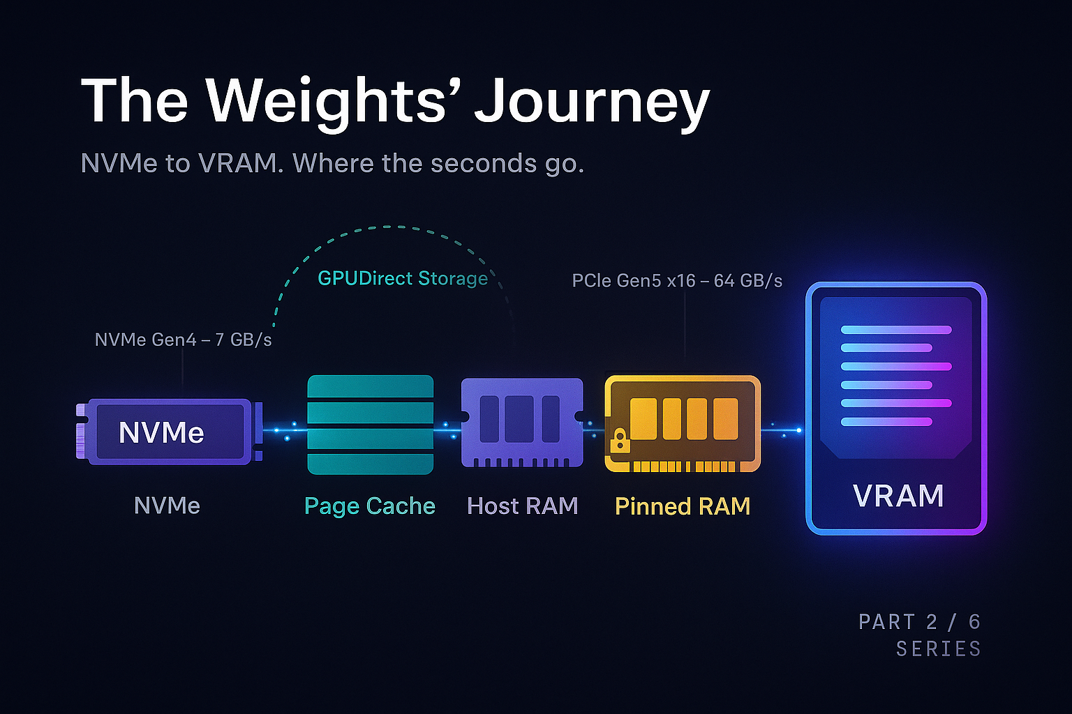
When you call from_pretrained() for a Llama 3 70B model on an H100 server, the weights travel a specific path:

Each stage has a bandwidth ceiling that limits performance.

A Gen4 NVMe drive reads at roughly 7 GB/s. Moving 140 GB takes at least 20 seconds. While Gen5 drives double this speed, the physical disk remains a primary constraint unless data is striped across multiple drives.

The Linux page cache significantly speeds up warm starts. The first read pulls from disk to RAM; subsequent reads access RAM at hundreds of GB/s. Cold start performance is disk-to-GPU, while warm start is RAM-to-GPU.

The PCIe Gen5 x16 link to an H100 peaks at 64 GB/s, typically reaching 50 to 55 GB/s in practice. Transferring 140 GB takes about 3 seconds. However, if data isn't in pinned memory, the driver must use a bounce buffer, potentially halving the bandwidth.

Pinned memory is host RAM that cannot be swapped out, allowing the GPU's DMA engine to read it directly. While tools like pin_memory=True enable this, pinned memory is a limited resource as it consumes physical RAM permanently.

mmap allows skipping the userspace copy. By mapping a safetensors file to virtual addresses, the library can issue a cudaMemcpyAsync directly from the page cache to the GPU, minimizing overhead.

Once your bytes arrive on the GPU, they have to live somewhere. The somewhere is allocated by the CUDA memory allocator.

PyTorch uses a caching allocator with a free list to wrap cudaMalloc. Since raw allocation is slow and synchronizes with the driver, reusing memory from a free list is much faster.

The downside is fragmentation. Scattered allocations can prevent large contiguous requests even if total free memory is high, leading to CUDA out of memory errors.

The first version of vLLM (Kwon et al., 2023) noticed that even with a good allocator, the way the KV cache is allocated leads to enormous fragmentation, and they responded by managing GPU memory themselves with a paged allocator modeled on virtual memory. We will return to this in Part 4.

Now we can finally answer the question: where do the seconds go? A naive PyTorch model load does roughly this:

1. Read the safetensors index from disk, figure out which shards exist.
2. For each shard, sequentially: open the file, parse the header, then for each tensor in the header - allocate a CPU tensor of the right shape and dtype, read the bytes into it, copy to GPU, free the CPU tensor.
3. Assemble all the tensors into a model state dict.
4. Call model.load_state_dict(state_dict) which does another round of copies into the actual model parameters.

Naive loaders suffer from sequential reads, redundant CPU copies, unpinned buffers, and lack of overlap between disk I/O and PCIe transfers. Loading a 70B model this way takes around 30 seconds, with at least 50% overhead from inefficient copying.

You can measure this. Loading Llama 3 70B from a warm page cache on a server with one H100, the naive path takes around 30 seconds. This high latency is not exclusive to large models; a direct PyTorch implementation of an 8B parameter model has been observed with 30-second query latency. Almost all of it is the PCIe transfer, but redundant copying easily adds 50% overhead.

Modern loaders utilize five key techniques.

GPUDirect Storage (GDS) removes the "host RAM" step, allowing the GPU to read directly from NVMe. This reduces CPU load and host bandwidth contention, though it requires specific driver and filesystem support.

GDS is most beneficial when host RAM is a bottleneck or when models are too large to stage through RAM effectively.

In production, cold starts impact user experience and costs. Three settings make it acute.

Autoscaling. If your traffic doubles and you spin up a new replica, the user requests that hit the new replica wait for the model to load. For a 70B model this is 30 seconds to a minute. The first users on the new replica see a 30 second TTFT. You can paper over this with warm pools (keeping spare replicas pre-loaded), but warm pools cost money even when idle.

Serverless inference. Modal, Banana, Replicate, and similar platforms charge by the second, so they aggressively spin GPUs down between requests. Every cold start is a user-visible latency hit. The serverless inference vendors have invested heavily in fast loaders precisely because their business depends on cold start being measured in seconds, not minutes.

Multi-tenant serving. If you serve many fine tuned variants of a base model, you cannot keep them all hot. You need to swap models in and out. The faster you can load, the more variants you can support on the same hardware.

The state of the art as of early 2026 is roughly:

The physical PCIe ceiling remains the ultimate limit, though hardware like NVIDIA Grace Hopper (using NVLink-C2C) provides a different path. For most, the goal is simply reaching that ceiling by eliminating software overhead.

Model loading is a "plumbing" problem with massive room for optimization. By removing hops between disk and VRAM and overlapping transfers, we can move closer to theoretical hardware limits.

In Part 3, we'll assume the weights are loaded and trace the flow of a single token through the network.

• Hugging Face safetensors specification: github.com/huggingface/safetensors
• llama.cpp GGUF specification: ggml/docs/gguf.md
• NVIDIA GPUDirect Storage documentation: docs.nvidia.com/gpudirect-storage
• PyTorch CUDACachingAllocator source: pytorch/c10/cuda/CUDACachingAllocator.cpp
• Kwon et al., 2023. "Efficient Memory Management for Large Language Model Serving with PagedAttention." SOSP 2023. arXiv:2309.06180.
• CoreWeave tensorizer: github.com/coreweave/tensorizer